- Published on
An Overview of the Singapore Hiring Landscape
- Authors
- Name
The idea of having a 360 degree view of the entire job seeking and matching landscape has always been a dream of any labour economist. Just imagine, a dataset of CVs and job seekers matched with job advertisements and openings! The potential of such a dataset to answer existing questions on the labour market is incredible. One could investigate market power between worker and firms, information asymmetry within the matching process, or find out new growth clusters and skills needed to support these areas. So it was slightly unfortunate that I was not able to get my hands on such a dataset during my time in the government (I believe only Linkedin could capture something close to what I described).
A few months ago, I decided to make some steps towards creating that dream dataset. While getting information on the candidate side is near impossible, data on job openings are readily available through job portals. Over a few weekends, I wrote a scrapy bot to crawl and save job postings from one major Singapore based job portal.1 Having collected a full month of data for October, I thought it was a good opportunity to carry out an exploratory analysis of the dataset. This post features that analysis along with some tidbits of the Singapore hiring landscape. If anyone is interested in studying this dataset in more detail, feel free to drop me an email!
Dataset
The job posting data is collected on a MySQL database and I will be using R along with the dbplyr package to explore the dataset. To interface with the backend database, I am using DBI to create a connection to it. For this post I created a slightly modified copy of the data in a table called sg_jobs_tbl.
For reference, the main fields that were scraped are the job title, posting date, company, post type (sponsored or not), occupation (called tag in the database), job description, experience required, company's address, company's industry and a brief overview of the company.
Data Cleaning
Let us begin by importing the libraries we require and setting up the database connection:
library(DBI)
library(tidyverse)

con <- dbConnect(RMariaDB::MariaDB(),
                 default.file	= paste0(path, '/.my.cnf'),
                 groups = 'jobs_db')
To query the database, we can use the dbSendQuery() function and pass in a standard sql statement for it to evaluate. dbFetch() is used to get the results back in a dataframe. Let's take a look at how many postings we have collected over the month of October:
q <- dbSendQuery(con, "SELECT count(*) FROM sg_jobs_tbl")
##   count(*)
## 1    55456
dbFetch(q)
dbClearResult(q)
We have more than 50,000 postings in a month, but how many of them are from recruiting agencies or direct job openings? We can filter out firms with 'recruitment firm' as part of their company description to derive the count of postings by actual companies.
q <- dbSendQuery(con, "SELECT count(*) FROM sg_jobs_tbl where company_snapshot not like '%RECRUITMENT FIRM%'")
##   count(*)
## 1    19327
dbFetch(q)
dbClearResult(q)
Apparently more than 50% of all job posts are by recruitment firms. This means that we have to be a little careful of the data quality since firms might spam the job board with multiple posts across the month for a single job opening.
One of the nice features of R is the tidyverse ecosystem. It provides a consistent syntax to manipulate data regardless of the backend source. So we can just use our favourite dplyr verbs and the package will automatically convert it to sql syntax.2 In the code below, I extract the most frequent company, title combinations across the entire month:
q <- tbl(con, "sg_jobs_tbl") %>%
  filter(!is.na(company), !is.na(title)) %>%
  group_by(company, title) %>%
  count() %>%
  arrange(desc(n))
A nice aspect of writing sql statements in dplyr syntax is that it is lazily evaluated i.e. the code will only be run when it is explicitly required, such as a print statement. Given a tbl object with a DBI connection, dplyr will use dbplyr to generate the sql translation which we can preview by calling the show_query() function. Even when we ask it to print the results of the query, it only returns the first 10 observations. To return the entire query as a data frame we have to use the collect() function. We can take advantage of this feature by just printing the query and getting the top 10 observations:
q
## # Source:     lazy query [?? x 3]
## # Database:   mysql 8.0.12 [root@localhost:/jobs_db]
## # Groups:     company, title
## # Ordered by: desc(n)
##    company                  title                                n
##    <chr>                    <chr>                                <S3: int>
##  1 ScienTec Personnel       ""                                   32
##  2 ST Electronics (Info-co~ Carpark Patrolling Officer     Ref ~ 24
##  3 Talentvis Singapore Pte~ Recruitment Consultant x2 (No exper~ 22
##  4 Dynamic Human Capital P~ Patient Service Associate x 20 ( Va~ 21
##  5 Achieve Career Consulta~ Wealth Manager x 5 / Top Foreign Ba~ 21
##  6 PRIMESTAFF MANAGEMENT S~ **Technology Assistant (up to $2300~ 18
##  7 JOBSTUDIO PTE LTD        Assistant Teachers x 10 (Childcare ~ 18
##  8 ST Electronics (e-Servi~ Audit Associate [W]                  16
##  9 ST Electronics (e-Servi~ Audit Associate (SDL VP Call) [W]    16
## 10 ST Electronics (e-Servi~ Customer Service Officer [CCAS - Bu~ 16
## # ... with more rows
Does ST Electronics really need 32 carpark officers? Let's take a look at the date which these offers are posted.
q <- tbl(con, "sg_jobs_tbl") %>%
  filter(company == 'ST Electronics (Info-comm Systems) Pte Ltd') %>%
  filter(title %like% '%Carpark Patrolling Officer%') %>%
  arrange(posted_dt) %>%
  select(posted_dt)

q
## # Source:     lazy query [?? x 1]
## # Database:   mysql 8.0.12 [root@localhost:/jobs_db]
## # Ordered by: posted_dt
##    posted_dt
##    <dttm>
##  1 2018-10-04 00:27:56
##  2 2018-10-13 00:12:24
##  3 2018-10-13 00:12:27
##  4 2018-10-13 00:12:27
##  5 2018-10-13 00:12:29
##  6 2018-10-13 00:12:29
##  7 2018-10-13 00:12:30
##  8 2018-10-13 00:12:31
##  9 2018-10-13 00:12:33
## 10 2018-10-13 00:12:36
## # ... with more rows
There appears to be numerous duplicated postings around midnight. This could possibly be a system issue. It is harder to tell whether jobs posted in different days across the month are actually for the same position or a different opening. For this analysis, we will just consider unique job postings in a single day. Again, we will make use of the lazy evaluation feature by creating an intermediate table called 'view' which all subsequent queries will be based off. Let's take another look at the most popular company, title combinations:
view <- tbl(con, "sg_jobs_tbl") %>%
  mutate(posted_dt = sql('date(posted_dt)')) %>%
  select(title, posted_dt, company, post_type, tag, jd, experience, address,
         company_industry, company_snapshot, company_overview) %>%
  distinct() %>%
  filter(!is.na(company), !is.na(title), title!="") %>%
  rename(occupation = tag)

q <- view %>%
  group_by(company, title) %>%
  count() %>%
  arrange(desc(n))

q
## # Source:     lazy query [?? x 3]
## # Database:   mysql 8.0.12 [root@localhost:/jobs_db]
## # Groups:     company, title
## # Ordered by: desc(n)
##    company                title                                  n
##    <chr>                  <chr>                                  <S3: int>
##  1 Dynamic Human Capital~ Patient Service Associate x 20 ( Vari~ 21
##  2 Achieve Career Consul~ Wealth Manager x 5 / Top Foreign Bank~ 21
##  3 Talentvis Singapore P~ Recruitment Consultant x2 (No experie~ 20
##  4 JOBSTUDIO PTE LTD      Assistant Teachers x 10 (Childcare / ~ 18
##  5 PRIMESTAFF MANAGEMENT~ **Technology Assistant (up to $2300 /~ 18
##  6 ST Electronics (e-Ser~ Claims Associate [W] (1 Year Contract) 15
##  7 ST Electronics (e-Ser~ Audit Associate [W]                    15
##  8 ST Electronics (e-Ser~ Audit Associate (SDL VP Call) [W]      15
##  9 ST Electronics (e-Ser~ Customer Service Officer [CCAS - Buki~ 15
## 10 ST Electronics (e-Ser~ Contact Centre Officer [W]             15
## # ... with more rows
The first 5 entries are recruitment firms with ST Electronics making up the rest of the top 10.
Exploratory Analysis
Which firms are hiring aggresively in October?
q <- view %>%
  filter(!(company_snapshot %like% '%RECRUITMENT FIRM SNAPSHOT%')) %>%
  group_by(company) %>%
  count() %>%
  arrange(desc(n))

top_hiring_companies <- collect(q)
head(top_hiring_companies, 15) %>% knitr::kable()
| company | n |
|---|---|
| National University of Singapore | 380 |
| ST Electronics (e-Services) Pte Ltd | 285 |
| United Overseas Bank Limited (UOB) | 255 |
| Micron Semiconductor Asia Pte Ltd | 194 |
| Nanyang Technological University | 159 |
| Government Technology Agency of Singapore (GovTech) | 156 |
| Certis CISCO Security Pte Ltd | 150 |
| ST Electronics (Info-Comm Systems) Pte Ltd | 129 |
| Marina Bay Sands Pte Ltd | 123 |
| Citi | 110 |
| Tan Tock Seng Hospital | 108 |
| Mediacorp Pte Ltd | 86 |
| Infineon Technologies | 80 |
| Singapore Airlines | 78 |
| Singapore Technologies Marine Ltd | 78 |
Not surprisingly, we have the government linked companies high in the list with NUS, ST Electronics and UOB in the top 3. The list also gives a preview on which industries have a shortage of workers and the skills that are in demand, namely, healthcare, engineering and IT.
Which industries have the most vacancies to fill?
q <- view %>%
  filter(!(company_snapshot %like% '%RECRUITMENT FIRM SNAPSHOT%')) %>%
  group_by(company_industry) %>%
  count() %>%
  arrange(desc(n))

top_hiring_industries <- collect(q)

top_hiring_industries <- top_hiring_industries %>%
  mutate(industry = strsplit(company_industry, split='/')[[1]][1])

top_hiring_industries %>%
  head(10) %>%
  ggplot(aes(x=industry, y=as.numeric(n), fill=as.factor(industry))) +
  geom_bar(stat = 'identity') +
  theme(axis.text.x=element_text(angle=45,hjust=1,vjust=1),
        axis.title.x=element_blank()) +
  theme_bw() +
  coord_flip() +
  scale_fill_brewer(guide=FALSE, palette ="Set3") +
  scale_x_discrete(limits = top_hiring_industries[['industry']][10:1]) +
  labs(y = 'Number of Job Postings', x = 'Industry',
       title = 'Number of Job Postings by Industry')
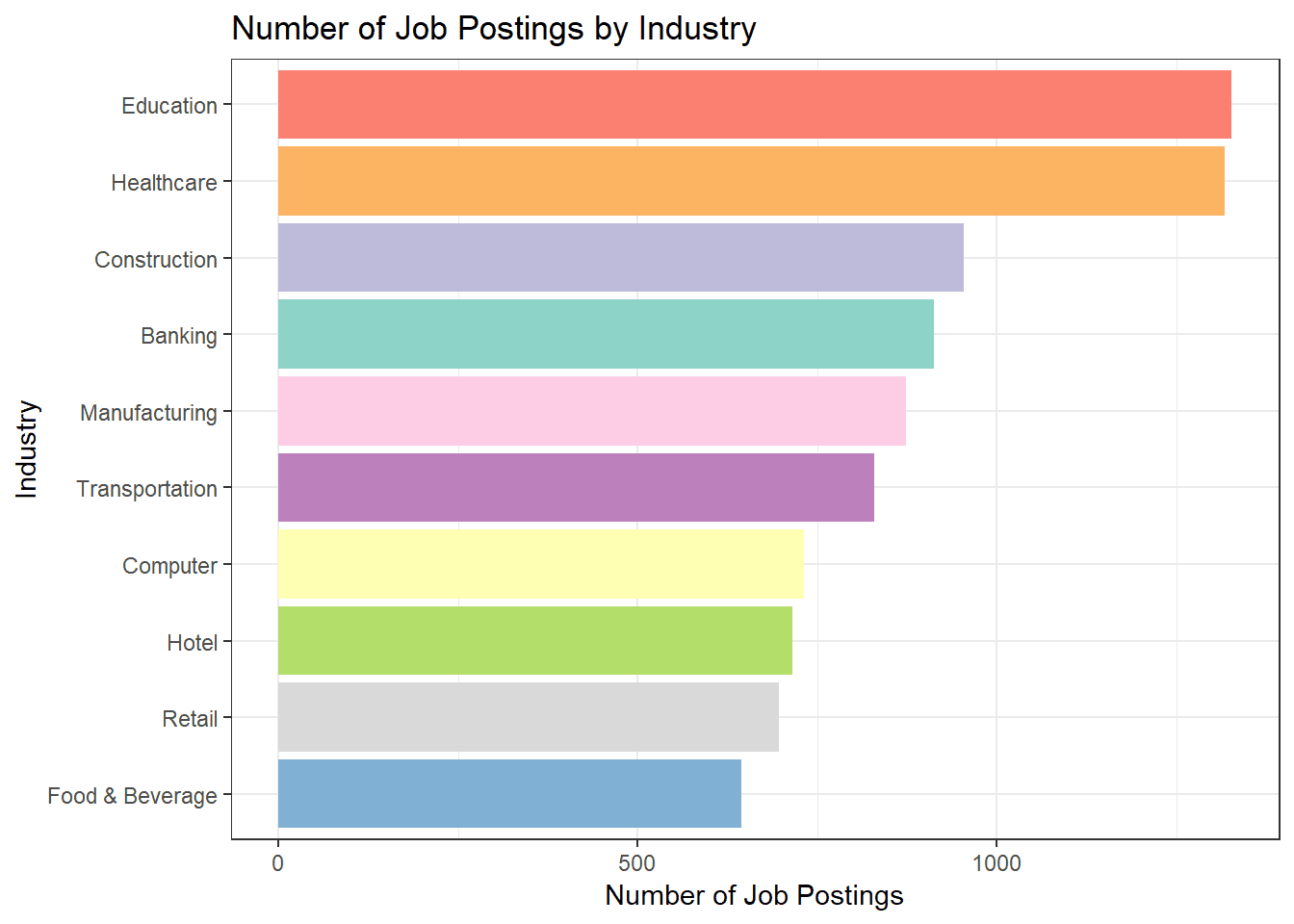
Let's examine the difference between the job posting statistics and the official employment numbers as published by the Department of Statistics quarterly statistics (You can take a look at my SG economy dashboard). Certain industries such as transportation, banking, education and healthcare are in line with the national employment trend. Interestingly, there is still quite a strong demand from the construction and manufacturing industry despite the negative outlook within those sectors. The discrepancy could be a result of structural mismatch between the workers that are laid off and the type of workers which those firms are looking to hire.
How does firm size correlate with hiring?
top_hiring_companies %>%
  mutate(posts = case_when(
    n >= 200 ~ '>= 200',
    n >= 100 ~ '100 - 200',
    n >= 50 ~ '50 - 100',
    n >= 25 ~ '25 - 50',
    n >= 10 ~ '10 - 25',
    n >= 5 ~ '5 - 10',
    n >= 3 ~ '2 - 5',
    n >= 1 ~ '1'
  )) %>%
  group_by(posts) %>%
  summarise(count = sum(n) / 1000) %>%
  arrange(desc(count)) %>%
  ggplot(aes(x=posts, y=as.numeric(count), fill = as.factor(count))) +
  geom_bar(stat = 'identity') +
  theme_bw() +
  scale_fill_brewer(guide=FALSE, palette ="Set3") +
  scale_x_discrete(limits = c('1', '2 - 5', '5 - 10', '10 - 25', '25 - 50',
                              '50 - 100', '100 - 200', '>= 200')) +
  labs(y = 'Sum of posts (thousands)', x = 'Firm Size (using posts as proxy)',
       title = 'Job Postings by Firm Size')
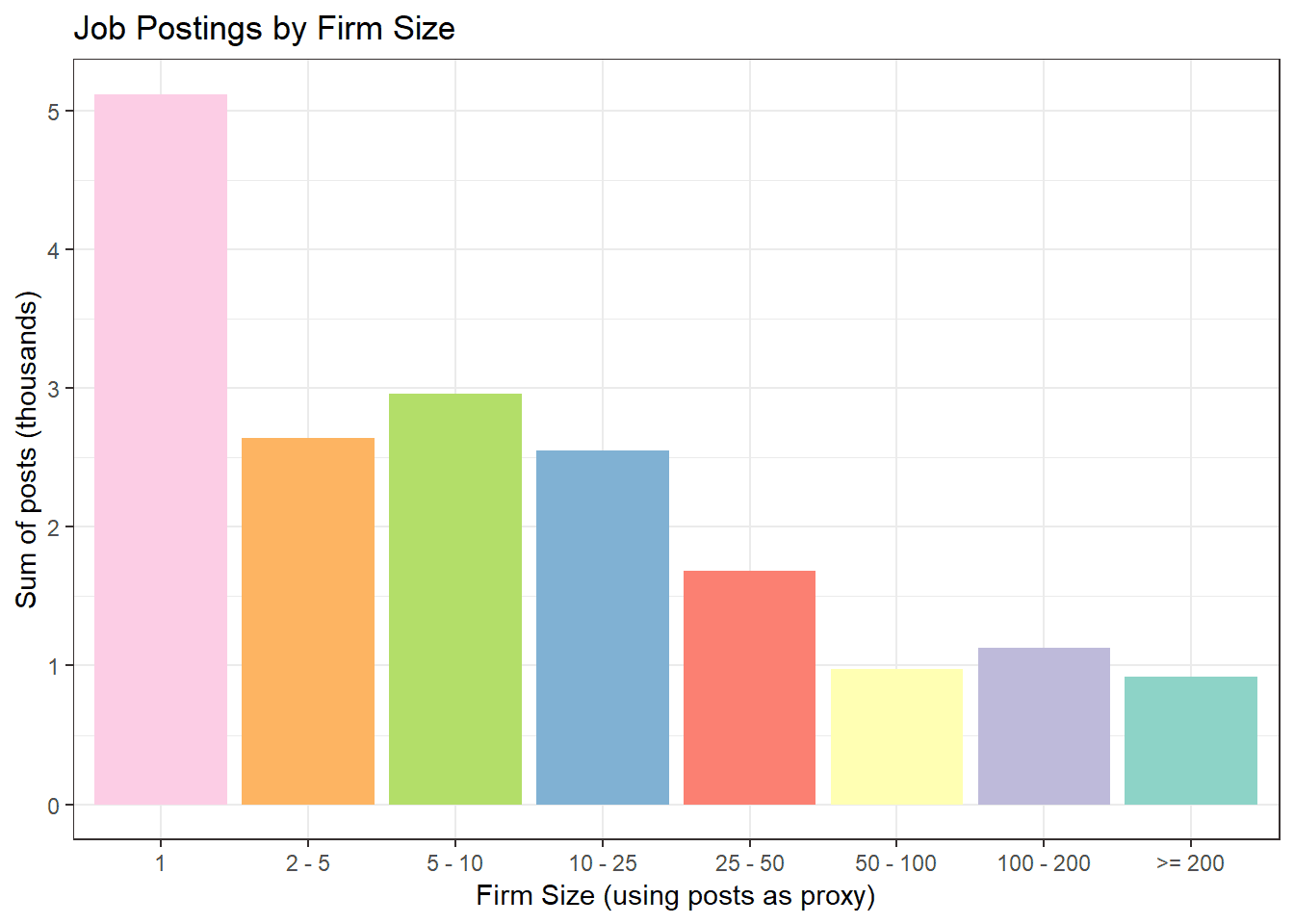
We can use the number of post as a proxy for the size of the firm (larger firms have more open positions). Firms which are aiming to hire less than or equal to 10 people, contribute to more than 50% of the total potential hiring. There are about 5000+ firms looking to fill only a single vacancy.
Which job positions are most in demand?
q <- view %>%
  filter(!(company_snapshot %like% '%RECRUITMENT FIRM SNAPSHOT%'),
         !is.na(occupation)) %>%
  group_by(occupation) %>%
  count() %>%
  arrange(desc(n))

top_vacancies <- collect(q)
nrow(top_vacancies)
## [1] 6163
head(top_vacancies, 15) %>% knitr::kable()
| occupation | n |
|---|---|
| senior | 347 |
| executive | 336 |
| manager | 325 |
| assistant manager | 228 |
| sales executive | 211 |
| senior executive | 176 |
| customer service officer | 156 |
| senior manager | 151 |
| project manager | 127 |
| vp | 124 |
| admin assistant | 122 |
| accounts executive | 116 |
| marketing executive | 95 |
| accountant | 94 |
| research fellow | 94 |
Most of the positions are generic titles or business support positions that cut across industries. In total, there are more than 6,000 unique occupations listed.
Recruitment firms vs direct openings?
q <- view %>%
  mutate(recruiter = ifelse(company_snapshot %like% '%RECRUITMENT FIRM SNAPSHOT%', 1, 0)) %>%
  group_by(occupation, recruiter)  %>%
  count()

jobs_source_count <- collect(q)

q <- view %>%
  group_by(occupation) %>%
  summarise(count_total = n()) %>%
  filter(count_total >= 5)

jobs_count <- collect(q)

direct_jobs <- jobs_count %>%
  inner_join(jobs_source_count, by = 'occupation') %>%
  mutate(frac = n / count_total) %>%
  filter(recruiter == 0) %>%
  arrange(desc(frac), desc(count_total))

indirect_jobs <- jobs_count %>%
  inner_join(jobs_source_count, by = 'occupation') %>%
  mutate(frac = n / count_total) %>%
  filter(recruiter == 1) %>%
  arrange(desc(frac), desc(count_total))

compare_jobs <- jobs_count %>%
  inner_join(jobs_source_count, by = 'occupation') %>%
  mutate(frac = n / count_total) %>%
  filter(recruiter == 1, frac > 0.1, frac < 0.9, count_total > 50) %>%
  arrange(desc(frac)) %>%
  select(occupation, count_total, frac)

head(compare_jobs, 10) %>% knitr::kable()
| occupation | count_total | frac |
|---|---|---|
| admin | 59 | 0.8983051 |
| desktop engineer | 56 | 0.8928571 |
| internal auditor | 52 | 0.8846154 |
| shipping assistant | 51 | 0.8823529 |
| it project manager | 51 | 0.8823529 |
| beauty advisor | 73 | 0.8767123 |
| product specialist | 63 | 0.8730159 |
| production technician | 86 | 0.8720930 |
| bim modeller | 53 | 0.8679245 |
| warehouse assistant | 315 | 0.8666667 |
tail(compare_jobs, 10) %>% knitr::kable()
| occupation | count_total | frac |
|---|---|---|
| senior executive | 265 | 0.3358491 |
| senior engineer | 76 | 0.3026316 |
| manager | 462 | 0.2965368 |
| administrative assistant | 82 | 0.2682927 |
| assistant director | 81 | 0.2469136 |
| executive | 442 | 0.2352941 |
| associate | 85 | 0.2235294 |
| avp | 110 | 0.2181818 |
| technical officer | 62 | 0.1451613 |
| vp | 138 | 0.1014493 |
The fractions in the table above refers to the fraction of jobs that are posted by recruitment firms. From the first table, we see that a lot of admin and IT related positions are typically filled with the help of recruitment firms. Companies prefer to source for more senior positions directly and they tend to use more generic titles when creating job openings.
This post is a first look at a dataset of job openings. Besides the fields discussed in the exploratory analysis, there remains two other free text fields, job description and company description, which could be analysed in greater detail. I have many other ideas to explore with this dataset so do check back or subscribe to the RSS feed for future updates.