- Published on
Schelling's Segregation Model in Julia
- Authors
- Name

This article is the first of a series that introduces the Julia programming language by replicating Schelling, Thomas C. "Dynamic models of segregation." Journal of mathematical sociology 1.2 (1971): 143-186.
Follow along by cloning the git repository over here: https://github.com/timlrx/learning-julia
Why Julia?
From the creator's themselves:
We are greedy: we want more.
We want a language that's open source, with a liberal license. We want the speed of C with the dynamism of Ruby. We want a language that's homoiconic, with true macros like Lisp, but with obvious, familiar mathematical notation like Matlab. We want something as usable for general programming as Python, as easy for statistics as R, as natural for string processing as Perl, as powerful for linear algebra as Matlab, as good at gluing programs together as the shell. Something that is dirt simple to learn, yet keeps the most serious hackers happy. We want it interactive and we want it compiled.
I like ambitious projects and have been looking for a more performant language for a while. Benchmark comparisons seem really good - I even wrote one a few months ago comparing graph packages! - so I thought it would be fun to test it out on a project.
This week's Juliacon was also quite inspiring and they were nice enough to make it free to join so here's a way to pay it forward and introduce to everyone the wonders and idiosyncrasies of Julia.
Why Schelling's Model?
Personally, it was one of the studies that enticed me to study economics. I came across the model while reading Schelling's Micromotives and Macrobehavior. Here are two of my favourite quotes from the book:
Models tend to be useful when they are simultaneously simple enough to fit a variety of behaviors and complex enough to fit behaviors that need the help of an explanatory model
An equilibrium is simply a result. It is what is there after something has settled down, if something ever does settle down . . . The body of a hanged man is in equilibrium when it finally stops swinging, but nobody is going to insist that the man is all right.
It's a classical paper in the social science literature with wide influence in urban studies, economics, sociology among other disciplines. The model is brilliantly simple - one could replicate it with a checkers board set, with remarkably profound conclusions.
Why another tutorial?
There are many other tutorials and introductory material out there that I recommend and have learnt from:
- The Reference Docs
- Quantitative Economics with Julia
- From Zero to Julia
- Julia for Data Science
- And many others...
I take a slightly different approach. Rather than going over concepts (Types, Loops, Control Statements etc.), I take a problem-driven approach - given a particular problem, how can we solve it using Julia. This is my favourite way to learn something new, try it on an actual problem and see where we end up!
Pre-requisites and Setup
Some prior experience in languages like Python or R and knowledge of git would be useful.
For development, this code is written in Julia v1.4, using both the Jupyter Notebook interface as well as the vscode plugin for editing .jl files.
Follow the instructions over here to set up Jupyter for Julia and julia-vscode plugin.
Let's get started!
This is mostly a walkthrough of the notebook, with a more detailed description of the findings. Feel free to clone the repository and follow along!
Note: This is not meant to demonstrate how to write high performance or even good Julia code. Our first notebook shows how easy it is to get started. You will see many similarities to Python - no types need to be specified and pick up some nice syntactical properties of Julia. Some parts of the post go into more programming related intricacies - I prepend those with a Julia Internals tag. Feel free to skip over those paragraphs or revisit them another day.
Just like Python or R, we start off by importing the packages we need. We can just import all the functions of a package by calling using StatsBase or import specific functions by calling using StatsBase: sample to import only the sample function.
using Revise
using Parameters, LinearAlgebra, Statistics, StatsPlots, DataFrames
using StatsBase: sample, countmap
using DataStructures: OrderedDict
If you encounter an error like ArgumentError: Package Revise not found in current path, please add the packages to your environment:
- Run
import Pkg; Pkg.add("Revise")to install the Revise package; - Or go into the package manager in the REPL by typing
]and adding the package withadd Revise
Linear Model
To implement the model, we need to define a neighborhood and its agents.1
Setup
- Agents
- kind of agent (stars or circle)
- location
- preferences (conditions which agent is satisfied)
- Neighborhood
- Agents
- location
- size
We can use Structs to define a collection of interest.
Julia Internals: Structs are a collection of named fields similar to classes in Python, interfaces in typescript or structs in C. The main difference in Julia is that functions are not bundled with the objects they operate on. Instead, functions and even constructors tend to live outside the struct. This is one of the main differentiating factors of Julia which we will explore in a subsequent post. If you are interested to learn more about structs, check out the official documentation on Composite Types.
The @Base.kwdef macro allows us to use keywords to define the struct. This is our first encounter of a Julia macro!
mutable struct Agent
   id
   kind
   location
   neighborhood_size   # Max neighborhood distance to consider to determine share preference
   preference          # Preference ratio for the Agent to be happy
end
@Base.kwdef mutable struct Neighborhood
   agents
   locations
   size
end
Having defined our objects or structs, we can create instances of them as follows. With the keyword structs, we can define them using keyword arguments instead of positional arguments.
a1 = Agent(1, "Stars", 2, 4, 0.5)
a2 = Agent(2, "Circle", 3, 4, 0.5)
nh1 = Neighborhood(agents=[a1, a2], locations=Dict(a1 => 2, a2 => 3), size=2)
Three things to note in the following code block:
Functions in Julia are very similar in style to Python. The main thing to note is that they do not rely on whitespace to denote blocks. Instead, one has to append an
endat the end of the function to close it. If / else statements are written similarly as well.Docstrings are written above the function instead of inside it.
There's a built-in pipe operator
|>, which makes chaining functions fun and readable!Julia has a convention where functions ending with ! modifies their arguments. So
push!functions modifies the array which we are pushing an object to.
# Docstring in Julia is written above the function as shown below

"Initializes the neigbourhood by mapping a dictionary of agent types to population size."
function init_neighborhood(population_dict, neighborhood_size, preference)

    # Pipe operator |>, equivalent to: sum(collect(values(agent_number)))
    # Similar to R's %>%
    n = population_dict |> values |> collect |> sum
    location_dict = Dict()

    # Create a list of agents
    pos = sample(1:n, n, replace=false)
    agents = []
    counter = 0
    for (key, value) in population_dict
        for i in 1:value
            id = i + counter
            new_agent = Agent(id, key, pos[id], neighborhood_size, preference)

            # Julia has a convention where functions ending with ! modifies their arguments
            # In this case we are inserting a new_agent into the agents list
            push!(agents, new_agent)
            location_dict[pos[id]] = new_agent
        end
        counter += value
    end
    return Neighborhood(agents=agents, locations=location_dict, size=n)
end
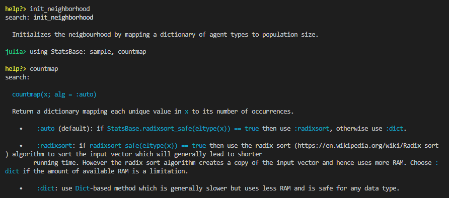
Need help?
Use the '?' sign to get information about a function or an object - similar to R. Here's an example on the function we have previously defined and countmap which we will use later on in the tutorial.
?init_neighborhood
?countmap
Let's give our init_neighborhood function a test run.
population_dict = Dict("Stars"=>2, "Circle"=>2)
nh = init_neighborhood(population_dict, 4, 0.5)
Neighborhood(Any[Agent(1, "Stars", 3, 4, 0.5), Agent(2, "Stars", 4, 4, 0.5), Agent(3, "Circle", 1, 4, 0.5), Agent(4, "Circle", 2, 4, 0.5)], Dict{Any,Any}(4 => Agent(2, "Stars", 4, 4, 0.5),2 => Agent(4, "Circle", 2, 4, 0.5),3 => Agent(1, "Stars", 3, 4, 0.5),1 => Agent(3, "Circle", 1, 4, 0.5)), 4)
Instead of writing Dict("Stars"=>2, "Circle"=>2) we could have written Dict("⭐"=>2,"◯"=>2) Julia supports the use of unicode symbols which makes it nice to write math like operations.
We can suppress the final output by inserting a semicolon at the end of the statement. As in the original paper, let's create a neighborhood with 35 stars and 35 circles.2 Each person considers his neighbors living up to 4 doors away when evaluating his/her happiness.
# Suppress output with the semicolon;
nh = init_neighborhood(Dict("Stars"=>35, "Circle"=>35), 4, 0.5);
We are now going to sketch out the main logic of the agent-based modelling.
Iteration steps
- Mark out unhappy actors
- Use rule to decide how they move
- Move agents
- Repeat till everyone is happy / system converged
Schelling's rules
- Wants at least half of the neighbors to be of the same type
- Dissatisfied member move to the nearest point which he is satisfied
Here's a function to test whether an agent is happy or not. At a quick glance, you might have thought this is Python code - list comprehensions are part of Julia as well. An additional detail, we use the get function to return 0 if none of the neighbors is of the same type as the agent.
function is_happy(nh, agent_id)
    a = nh.agents[agent_id]
    neighbors = [
      [nh.locations[i] for i in max(a.location - a.neighborhood_size, 1):a.location-1];
      [nh.locations[i] for i in a.location+1:min(a.location + a.neighborhood_size, nh.size)]
    ]
    neighbors_kind = [a.kind for a in neighbors]
    cmap = countmap(neighbors_kind)
    share = get(cmap, a.kind, 0) / length(neighbors)  # If key does not exist, there are 0 of its kind
    return share ≥ a.preference
end
Let's test it out. We can use the handy @show macro to print out the statement as well as its evaluated contents.
@show a = nh.locations[2]
is_happy(nh, a.id)
a = nh.locations[2] = Agent(35, "Stars", 2, 4, 0.5) false
Julia Internals: This is the second macro that we came across. It might seem like jupyter magic commands, but it's even better than that. More generally metaprogramming
- the ability to represent code as a data structure of the language itself - is a native part of Julia. It allows the programmer to modify the code after it has been parsed to an abstract syntax tree but before it is evaluated.
Apparently, the agent living in location 2 (in my example) does not like his neighbors. Let's verify it with a plot.
Visualizing the neighborhood
StatsPlots should contain the dependencies needed for Plots, otherwise: Pkg.add("Plots")
In the plot neighborhood function below, we encounter 3 new Julia syntax:
Ternary operators like R or Javascript
a.kind == "Circle" ? :circle : :starAnnonymous functions as concise as Javascript arrow syntax:
x->x[1]Symbols e.g.
:circleor:orangewhich are 'special' strings that can be evaluated to values bound to it. Julia Internals: It's part of the metaprogramming aspect of Julia discussed above. For more information, check out the following helpful post: https://stackoverflow.com/questions/23480722/what-is-a-symbol-in-julia
function plot_nh(nh)
    ordered_loc = sort!(OrderedDict(nh.locations), by=x->x[1])
    m = [a.kind == "Circle" ? :circle : :star for a in values(ordered_loc)]
    c = [is_happy(nh, a.id) ? :lightblue : :orange for a in values(ordered_loc)]
    scatter(1:nh.size, ones(nh.size), color=c, m=m, markersize=6,
        axis=false, grid=false, ylimit=[0.8,1.2], legend=false, size=(1000,100))
end

plot_nh(nh)

Update Logic
Let's round up the main part of the program by writing out the update logic. To model an agent moving to the nearest location which meets his satisfaction criteria, we can just enumerate through the list of possible options in an alternating series (+1, -1, +2, -2 ... +70, -70). At each location, we attempt to move the agent there and shift the affected neighbours down / up. If the agent is not satisfied, we reverse the movement. Since this changes the neighborhood arrangement that is passed into the function, we append the exclamation symbol to the back of it.
As a side note, to reference the end of a vector, we use the end keyword e.g. options[end].
# Follow the use of exclamation mark since we are modifying nh

function update!(nh, agent_id)
    # Choose nearest new locations until happy.
    a = nh.agents[agent_id]
    original_location = a.location
    options = [i % 2 == 1 ? ceil(Int64, i/2) : ceil(Int64, -i/2) for i in 1:nh.size*2]
    for i in options
        attempt_location = original_location + i
        if (0 < attempt_location <= nh.size)
            # @show (original_location, attempt_location)
            move_location!(nh, a, attempt_location)
            if is_happy(nh, agent_id)
                break
            elseif (i==options[end])
                println(a, " Unable to find a satisfactory location")
            else
                # Revert
                move_location!(nh, a, original_location)
            end
        end
    end
end

function move_location!(nh, a, loc)
    # Update all other agents in between old location and new location
    update_seq = (loc > a.location) ?
        (a.location+1 : 1 : loc) :
        (a.location-1 : -1 : loc)

    # If the new location is higher everyone has to shift down
    for i in update_seq
        a2 = nh.locations[i]
        a2_new_location = (loc > a.location) ? i-1 : i+1
        a2.location = a2_new_location
        nh.locations[a2_new_location] = a2
    end

    # Move agent itself to new location
    a.location = loc
    nh.locations[loc] = a
end
Here's a way of calculating the fraction of people in the entire neighborhood who are happy with their current locations.
@show frac_happy =sum([is_happy(nh,i) for i in 1:nh.size])/ nh.size
frac_happy = sum([is_happy(nh, i) for i = 1:nh.size]) / nh.size = 0.6714285714285714
Results
We can combine the different functions we have created previously to capture the logic of Schelling's model in the run_simulation function. For each simulation cycle, we plot the end state of the neighborhood. The simulation ends when everyone is satisfied with their locations or if there is no change in the happiness score.3
Here, we also introduce the syntax in Julia which specifies whether a positional or keyword argument is accepted into a function. Everything to the left of the semicolon is a positional argument, while everything to the right is a keyword argument.
function run_simulation(agents=Dict("Stars"=>35, "Circle"=>35); neighborhood_size=4, preference=0.5)
    nh = init_neighborhood(agents, neighborhood_size, preference)
    plot_list = []
    prev_frac_happy = 0
    frac_happy = sum([is_happy(nh, i) for i in 1:nh.size]) / nh.size
    cycle = 1
    push!(plot_list, plot_nh(nh))
    while ((frac_happy < 1) && (cycle <= 10) && (prev_frac_happy != frac_happy))
        for i in 1:nh.size
            if !is_happy(nh, i)
                update!(nh, i)
            end
        end
        cycle += 1
        prev_frac_happy = frac_happy
        frac_happy = sum([is_happy(nh, i) for i in 1:nh.size]) / nh.size
        push!(plot_list, plot_nh(nh))
    end
    return nh, plot_list
end

function plot_results(results)
    n = length(results)
    plot(results...,
        layout = (n, 1),
        size = (1000, 100n),
        title = reshape(["Cycle $i" for i in 1:n], 1, n))
end

nh, results = run_simulation(Dict("Stars"=>35, "Circle"=>35), neighborhood_size=4, preference=0.5);
plot_results(results)
We have completed one run of our linear model and can visualise the migration process over the model's iteration! Is this run representative of a typical convergence process? How does changing an agent's neighborhood size or preference ratio affect the outcome? The following section explore these questions in more detail.
Varying parameters
Before we start running more iterations of the model, let's set up a way to capture certain key outcomes - the fraction of the population who are happy, whether the model has converged, the number of cycles it took and an overall diversity score metric. As a simple way of calculating a diversity score metric, we modify the is_happy function assuming that the social planner would like everyone equally mixed given a neighborhood size of 4.
"Fraction of neighbors not like yourself"
function diversity_score(nh, agent_id)
    neighborhood_size = 4
    a = nh.agents[agent_id]
    neighbors = [
      [nh.locations[i] for i in max(a.location - neighborhood_size, 1):a.location-1];
      [nh.locations[i] for i in a.location+1:min(a.location + neighborhood_size, nh.size)]
    ]
    neighbors_kind = [a.kind for a in neighbors]
    cmap = countmap(neighbors_kind)
    score = 1 - (get(cmap, a.kind, 0) / length(neighbors))
    return min(score / 0.5, 1) # 0.5 is the default agents max acceptable preference
end
function get_metric(simulation)
    nh, results = simulation
    frac_happy = sum([is_happy(nh, i) for i in 1:nh.size]) / nh.size
    has_converged = frac_happy == 1 ? true : false
    num_cycles = length(results) - 1 #Last plot shows final state
    score = sum([diversity_score(nh, i) for i in 1:nh.size]) / nh.size * 100
    return frac_happy, has_converged, num_cycles, score
end
We can store the results of 500 iterations using a list comprehension and calling the run_simulation function with our desired parameters.
experiment = [run_simulation(Dict("Stars"=>35, "Circle"=>35), neighborhood_size=4, preference=0.5) for i in 1:500];
To calculate our desired metrics on each run of the simulation, we use the broadcast operator or its alias the dot operator (f.x corresponds to broadcast(f, x)). It works similarly to the broadcast function in numpy if you are familiar with it.
Julia Internals: The broadcast operator is an alternative to Python / R vectorized operations which allows the caller to decide which function to vectorize and avoids any allocation of unnecessary temporary arrays. Nested dot calls are fused into a single loop which makes it much more performant. The nice thing about Julia is that every binary operation like +, has a corresponding dot operation e.g. .+. A statement like 2 .* x .+ x .^ 2 translates to broadcast(x -> 2*x + x^2, x). Check out this very informative blog post for more information: https://julialang.org/blog/2017/01/moredots/
We use the DataFrame library to collate the results and do some filtering and sorting to get the most diverse and least diverse scores.
df = get_metric.(experiment) |> DataFrame
rename!(df, ["frac_happy", "has_converged", "num_cycles", "score"])
df.row = axes(df, 1)
sort!(df, :score)
first(df, 3)
3 rows × 5 columns
| frac_happy | has_converged | num_cycles | score | row | |
|---|---|---|---|---|---|
| Float64 | Bool | Int64 | Float64 | Int64 | |
| 1 | 1.0 | 1 | 1 | 14.2857 | 187 |
| 2 | 1.0 | 1 | 2 | 21.4286 | 15 |
| 3 | 1.0 | 1 | 2 | 21.4286 | 315 |
last(df, 3)
3 rows × 5 columns
| frac_happy | has_converged | num_cycles | score | row | |
|---|---|---|---|---|---|
| Float64 | Bool | Int64 | Float64 | Int64 | |
| 1 | 0.957143 | 0 | 3 | 73.0816 | 434 |
| 2 | 0.971429 | 0 | 3 | 79.3027 | 125 |
| 3 | 0.985714 | 0 | 3 | 79.9354 | 303 |
How does a low diversity or high diversity neighborhood look like? It's quite incredible that starting with a preference of "not wanting to be the minority class", we could get outcomes where agents live in very polarized neighborhoods. An outcome which would satisfy everyone would be to simply alternate the circles and stars. Yet, the probability of that happening by random chance is close to zero.
lowest_diversity = filter(row -> row[:has_converged] == 1,df) |> first
_, results = experiment[lowest_diversity.row]
plot_results(results)

highest_diversity = filter(row -> row[:has_converged] == 1,df) |> last
_, results = experiment[highest_diversity.row]
plot_results(results)

Varying neighborhood size and preference ratio
We compare the baseline results against two alternate runs - one with a higher neighborhood consideration size and a second one with more tolerant agents (lower preference threshold).
experiment2 = [run_simulation(Dict("Stars"=>35, "Circle"=>35), neighborhood_size=8, preference=0.5) for i in 1:500];
df2 = get_metric.(experiment2) |> DataFrame
rename!(df2, ["frac_happy", "has_converged", "num_cycles", "score"]);

experiment3 = [run_simulation(Dict("Stars"=>35, "Circle"=>35), neighborhood_size=4, preference=0.3) for i in 1:500];
df3 = get_metric.(experiment3) |> DataFrame
rename!(df3, ["frac_happy", "has_converged", "num_cycles", "score"]);
describe(df)
5 rows × 8 columns
| variable | mean | min | median | max | nunique | nmissing | eltype | |
|---|---|---|---|---|---|---|---|---|
| Symbol | Float64 | Real | Float64 | Real | Nothing | Nothing | DataType | |
| 1 | frac_happy | 0.989257 | 0.942857 | 1.0 | 1.0 | Float64 | ||
| 2 | has_converged | 0.542 | 0 | 1.0 | 1 | Bool | ||
| 3 | num_cycles | 2.516 | 1 | 2.0 | 5 | Int64 | ||
| 4 | score | 47.2086 | 14.2857 | 50.0 | 79.9354 | Float64 | ||
| 5 | row | 250.5 | 1 | 250.5 | 500 | Int64 |
describe(df2)
4 rows × 8 columns
| variable | mean | min | median | max | nunique | nmissing | eltype | |
|---|---|---|---|---|---|---|---|---|
| Symbol | Float64 | Real | Float64 | Real | Nothing | Nothing | DataType | |
| 1 | frac_happy | 0.979486 | 0.885714 | 0.985714 | 1.0 | Float64 | ||
| 2 | has_converged | 0.472 | 0 | 0.0 | 1 | Bool | ||
| 3 | num_cycles | 3.166 | 1 | 3.0 | 5 | Int64 | ||
| 4 | score | 26.0721 | 7.14286 | 28.5714 | 43.5136 | Float64 |
describe(df3)
4 rows × 8 columns
| variable | mean | min | median | max | nunique | nmissing | eltype | |
|---|---|---|---|---|---|---|---|---|
| Symbol | Float64 | Real | Float64 | Real | Nothing | Nothing | DataType | |
| 1 | frac_happy | 0.941629 | 0.814286 | 0.942857 | 1.0 | Float64 | ||
| 2 | has_converged | 0.02 | 0 | 0.0 | 1 | Bool | ||
| 3 | num_cycles | 2.528 | 1 | 3.0 | 4 | Int64 | ||
| 4 | score | 77.8895 | 47.6531 | 79.0816 | 96.7857 | Float64 |
We can compare the distribution of scores across all 3 model runs using a density chart. With a larger neighborhood of consideration, we get less diversed communities as each agent is more concerned about the "broader neighborhood". Higher tolerance scores also lead to more diverse neighborhoods.
density(df.score, title="Diversity Scores with Varying NH Size and Preference", xaxis="Diversity Score", label="nh_size=4, p=0.5")
density!(df2.score, label="nh_size=8, p=0.5")
density!(df3.score, label="nh_size=4, p=0.3")

Varying neighborhood composition
Next, we run 3 other comparisons to explore how changing the underlying class composition might affect mixing.
experiment4 = [run_simulation(Dict("Stars"=>50, "Circle"=>50), neighborhood_size=4, preference=0.5) for i in 1:500];
df4 = get_metric.(experiment4) |> DataFrame
rename!(df4, ["frac_happy", "has_converged", "num_cycles", "score"]);

experiment5 = [run_simulation(Dict("Stars"=>35, "Circle"=>65), neighborhood_size=4, preference=0.5) for i in 1:500];
df5 = get_metric.(experiment5) |> DataFrame
rename!(df5, ["frac_happy", "has_converged", "num_cycles", "score"]);

experiment6 = [run_simulation(Dict("Stars"=>20, "Circle"=>80), neighborhood_size=4, preference=0.5) for i in 1:500];
df6 = get_metric.(experiment6) |> DataFrame
rename!(df6, ["frac_happy", "has_converged", "num_cycles", "score"]);
describe(df4)
4 rows × 8 columns
| variable | mean | min | median | max | nunique | nmissing | eltype | |
|---|---|---|---|---|---|---|---|---|
| Symbol | Float64 | Real | Float64 | Real | Nothing | Nothing | DataType | |
| 1 | frac_happy | 0.99296 | 0.96 | 1.0 | 1.0 | Float64 | ||
| 2 | has_converged | 0.582 | 0 | 1.0 | 1 | Bool | ||
| 3 | num_cycles | 2.506 | 1 | 2.0 | 4 | Int64 | ||
| 4 | score | 47.2306 | 25.0 | 45.8357 | 70.8476 | Float64 |
describe(df5)
4 rows × 8 columns
| variable | mean | min | median | max | nunique | nmissing | eltype | |
|---|---|---|---|---|---|---|---|---|
| Symbol | Float64 | Real | Float64 | Real | Nothing | Nothing | DataType | |
| 1 | frac_happy | 0.99436 | 0.96 | 1.0 | 1.0 | Float64 | ||
| 2 | has_converged | 0.66 | 0 | 1.0 | 1 | Bool | ||
| 3 | num_cycles | 2.208 | 1 | 2.0 | 5 | Int64 | ||
| 4 | score | 35.9291 | 15.0 | 35.8 | 55.3571 | Float64 |
describe(df6)
4 rows × 8 columns
| variable | mean | min | median | max | nunique | nmissing | eltype | |
|---|---|---|---|---|---|---|---|---|
| Symbol | Float64 | Real | Float64 | Real | Nothing | Nothing | DataType | |
| 1 | frac_happy | 0.98374 | 0.8 | 1.0 | 1.0 | Float64 | ||
| 2 | has_converged | 0.852 | 0 | 1.0 | 1 | Bool | ||
| 3 | num_cycles | 1.38 | 1 | 1.0 | 3 | Int64 | ||
| 4 | score | 16.2037 | 5.0 | 10.0 | 55.9667 | Float64 |
Despite keeping preference ratio's similar, overall diversity score ends up decreasing as class imbalance increases. Not only is segregation more extreme, minority clusters become larger as the minority itself shrinks. Basically, with fewer minority members, there would be lower probability of a growth node occuring. From the results, it appears that the minority class tends to flock to a single node and the system quickly converges.
density(df4.score, title="Diversity Scores with Varying Population Share", xaxis="Diversity Score", label="50/50")
density!(df5.score, label="65/35")
density!(df6.score, label="80/20")

Restricted Movement
What if we restrict the movement of agents to search up to a maximum of 25% of overall neighborhood size? We modify the available options in the update function to reflect the new rule.4
# Modify the update function such that the search options is limited to nh.size / 2

function update!(nh, agent_id)
    # Choose nearest new locations until happy.
    a = nh.agents[agent_id]
    original_location = a.location
    options = [i % 2 == 1 ? ceil(Int64, i/2) : ceil(Int64, -i/2) for i in 1:nh.size/2]
    for i in options
        attempt_location = original_location + i
        if (0 < attempt_location <= nh.size)
            # @show (original_location, attempt_location)
            move_location!(nh, a, attempt_location)
            if is_happy(nh, agent_id)
                break
            elseif (i==options[end])
            # println(a, " Unable to find a satisfactory location")
            else
                # Revert
                move_location!(nh, a, original_location)
            end
        end
    end
end
experiment4r = [run_simulation(Dict("Stars"=>50, "Circle"=>50), neighborhood_size=4, preference=0.5) for i in 1:500];
df4r = get_metric.(experiment4r) |> DataFrame
rename!(df4r, ["frac_happy", "has_converged", "num_cycles", "score"]);
describe(df4r)
4 rows × 8 columns
| variable | mean | min | median | max | nunique | nmissing | eltype | |
|---|---|---|---|---|---|---|---|---|
| Symbol | Float64 | Real | Float64 | Real | Nothing | Nothing | DataType | |
| 1 | frac_happy | 0.99242 | 0.96 | 1.0 | 1.0 | Float64 | ||
| 2 | has_converged | 0.542 | 0 | 1.0 | 1 | Bool | ||
| 3 | num_cycles | 2.556 | 1 | 3.0 | 5 | Int64 | ||
| 4 | score | 48.1284 | 25.0 | 50.0 | 75.5119 | Float64 |
experiment6r = [run_simulation(Dict("Stars"=>20, "Circle"=>80), neighborhood_size=4, preference=0.5) for i in 1:500];
df6r = get_metric.(experiment6r) |> DataFrame
rename!(df6r, ["frac_happy", "has_converged", "num_cycles", "score"]);
describe(df6r)
4 rows × 8 columns
| variable | mean | min | median | max | nunique | nmissing | eltype | |
|---|---|---|---|---|---|---|---|---|
| Symbol | Float64 | Real | Float64 | Real | Nothing | Nothing | DataType | |
| 1 | frac_happy | 0.99012 | 0.8 | 1.0 | 1.0 | Float64 | ||
| 2 | has_converged | 0.632 | 0 | 1.0 | 1 | Bool | ||
| 3 | num_cycles | 2.51 | 1 | 2.0 | 5 | Int64 | ||
| 4 | score | 18.9092 | 5.0 | 20.0 | 52.5381 | Float64 |
This results in higher diversity especially in neighborhoods where there is a class imbalance. One can see that the number of cycles and overall score is higher in experiment 6r compared to experiment 6. Intuitively, the restricted movement prevents a minority agent from joining large cliques and creates more growth clusters spread across the neighborhood.
Conclusion
We have successfully replicated the linear model in the paper and also created a framework which could be extended to other potential questions of interest - multiple classes, heterogenous agents etc.
If this is your first time seeing / writing Julia code - congratulations! In this first post, I hope you get a sense how similar and readable it is to Python. It allows for interactive computing and borrows many nice syntax from a variety of languages. There are packages available to work with dataframe like structures and the plotting package is excellent (much easier to learn than matplotlib).
In addition, we encountered some powerful features of the language like structs, broadcast operators and metaprogramming. In the next part of the series, I plan to show how we can transit to typed code and the performance benefits that comes along with it.
Footnotes
Getting the spelling of neighbors or neighbours right is the hardest part of the post. I hope I managed to make it consistent, but do forgive the inconsistencies if I slip into British English. ↩
Fun fact: In the original paper Schelling justifies the choice of 70 agents by claiming that it fits nicely within the margins of a typewriter and it is a large enough sample if both classes are in equal proportion. Thanks to modern day technology we can exceed the limit, but in the spirit of the paper we will still keep to 35 stars and circles! ↩
It is possible for the model to be stuck in a state where some agents can never be satisfied. For example, if there's an arrangement with 3 circles followed by 4 stars. The 3 circles would perpetually switch between themselves. ↩
The original paper adds a restriction on the travel distance as well as the movement rule. Keeping the movement rule the same, allows us to see the effect of only a restricted movement policy. ↩